Cats vs Dogs - Part 2 - 98.6% Accuracy - Binary Image Classification with Keras and Transfer Learning
May 12, 2019 -In 2014 Kaggle ran a competition to determine if images contained a dog or a cat. In this series of posts we'll see how easy it is to use Keras to create a 2D convolutional neural network that potentially could have won the contest.
In this post we'll see how we can fine tune a network pretrained on ImageNet and take advantage of transfer learning to reach 98.6% accuracy (the winning entry scored 98.9%).
In part 1 we used Keras to define a neural network architecture from scratch and were able to get to 92.8% categorization accuracy.
In part 3 we'll switch gears a bit and use PyTorch instead of Keras to create an ensemble of models that provides more predictive power than any single model and reaches 99.1% accuracy.
The code is available in a jupyter notebook here. You will need to download the data from the Kaggle competition. The dataset contains 25,000 images of dogs and cats (12,500 from each class). We will create a new dataset containing 3 subsets, a training set with 16,000 images, a validation dataset with 4,500 images and a test set with 4,500 images.
VGG16
We'll use the VGG16 architecture as described in the paper Very Deep Convolutional Networks for Large-Scale Image Recognition by Karen Simonyan and Andrew Zisserman. We're using it because it has a relatively simple architecture and Keras ships with a model that has been pretrained on ImageNet.
Keras includes a number of additional pretrained networks if you want to try with a different one. You could also build the VGG16 network yourself, the code for the Keras implementation is here. It is just a number of Conv2D and MaxPooling2D layers with a dense network on top with a final softmax activation function.
Predict what an image contains using VGG16
First we'll make predictions on what one of our images contained. The Keras VGG16 model provided was trained on the ILSVRC ImageNet images containing 1,000 categories. It will be especially useful in this case since it 90 of the 1,000 categories are species of dogs.
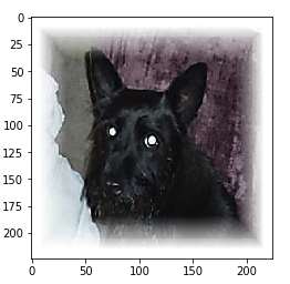
First lets take a peek at an image.
from keras.preprocessing import image
from matplotlib.pyplot import imshow

fnames = [os.path.join(train_dogs_dir, fname) for fname in os.listdir(train_dogs_dir)]
img_path = fnames[1] # Choose one image to view
img = image.load_img(img_path, target_size=(224, 224)) # load image and resize it
x = image.img_to_array(img) # Convert to a Numpy array with shape (224, 224, 3)

x = x.reshape((1,) + x.shape)

plt.imshow(image.array_to_img(x[0]))
Now lets ask the model what it thinks the picture is.
from keras.applications.imagenet_utils import decode_predictions
from keras.applications import VGG16

model = VGG16(weights='imagenet', include_top=True)

features = model.predict(x)
decode_predictions(features, top=5)
[[('n02097298', 'Scotch_terrier', 0.84078884),
  ('n02105412', 'kelpie', 0.07755529),
  ('n02105056', 'groenendael', 0.048816346),
  ('n02106662', 'German_shepherd', 0.006882491),
  ('n02104365', 'schipperke', 0.005642254)]]
It thinks there is an 84% chance it's a Scotch Terrier, and the other top predictions are all dogs. Seems pretty reasonable.
Train a Cats vs Dogs classifier
We can also ask Keras to provide us with the model trained on ImageNet, but without the top dense layers. Then it is just a matter of adding our own dense layers (note that since we are doing binary classification we've used a sigmoid activation function in the final layer). And tell the model to only train the dense layers we created (we don't want to retrain the lower layers that have learnt from ImageNet).
In this case it works so well because ImageNet has a large number of animal pictures, so the lower layers already have a sort of conception of what is "dogness" and "catness".
from keras import layers, models, optimizers


conv_base = VGG16(weights='imagenet',
                  include_top=False,
                  input_shape=(224, 224, 3))

model = models.Sequential()
model.add(conv_base)
model.add(layers.Flatten())
model.add(layers.Dropout(0.5))
model.add(layers.Dense(256, activation='relu'))
model.add(layers.Dense(1, activation='sigmoid'))

conv_base.trainable = False

model.compile(loss='binary_crossentropy',
              optimizer=optimizers.RMSprop(lr=2e-5),
              metrics=['acc'])
Lets create a generator for the images
from keras.applications.vgg16 import preprocess_input
from keras.preprocessing.image import ImageDataGenerator

train_datagen = ImageDataGenerator(preprocessing_function=preprocess_input)
test_datagen = ImageDataGenerator(preprocessing_function=preprocess_input)

# The list of classes will be automatically inferred from the subdirectory names/structure under train_dir
train_generator = train_datagen.flow_from_directory(
    train_dir,
    target_size=(224, 224), # resize all images to 224 x 224
    batch_size=50,
    class_mode='binary') # because we use binary_crossentropy loss we need binary labels

validation_generator = test_datagen.flow_from_directory(
    validation_dir,
    target_size=(224, 224), # resize all images to 224 x 224
    batch_size=50,
    class_mode='binary')
Found 16000 images belonging to 2 classes.
Found 4500 images belonging to 2 classes.
And train.
history = model.fit_generator(
    train_generator,
    steps_per_epoch=320, # batches in the generator are 50, so it takes 320 batches to get to 16000 images
    epochs=30,
    validation_data=validation_generator,
    validation_steps=90) # batches in the generator are 50, so it takes 90 batches to get to 4500 images
Epoch 1/30
320/320 [==============================] - 139s 434ms/step - loss: 0.7365 - acc: 0.9238 - val_loss: 0.2217 - val_acc: 0.9751
Epoch 2/30
320/320 [==============================] - 137s 428ms/step - loss: 0.2950 - acc: 0.9689 - val_loss: 0.2579 - val_acc: 0.9736
...
...
...
Epoch 29/30
320/320 [==============================] - 137s 429ms/step - loss: 0.0206 - acc: 0.9977 - val_loss: 0.2079 - val_acc: 0.9818
Epoch 30/30
320/320 [==============================] - 137s 429ms/step - loss: 0.0146 - acc: 0.9982 - val_loss: 0.2063 - val_acc: 0.9824
Lets take a look at what accuracy and loss looked like during training. The code to generate the plot is available in the posts jupyter notebook here.
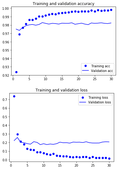
We seem to be overfitting (and probably could have trained for far fewer than 30 epochs), but the results are still pretty good. Lets compare against the holdout test set.
test_generator = test_datagen.flow_from_directory(
    test_dir,
    target_size=(224, 224),
    batch_size=50,
    class_mode='binary')

test_loss, test_acc = model.evaluate_generator(test_generator, steps=90)
print('test acc:', test_acc)
Found 4500 images belonging to 2 classes.
test acc: 0.9833333353201549
A validation accuracy of 98.2% and test of 98.3%. Not bad, but lets see if we can do better.
Transfer learning / Fine tune model
We can also retrain the later convolutional layers. Here is how we can do it with VGG16.
conv_base = VGG16(weights='imagenet',
                  include_top=False,
                  input_shape=(224, 224, 3))

conv_base.trainable = True

set_trainable = False
for layer in conv_base.layers:
    if layer.name == 'block5_conv1':
        set_trainable = True
    if set_trainable:
        layer.trainable = True
    else:
        layer.trainable = False


model = models.Sequential()
model.add(conv_base)
model.add(layers.Flatten())
model.add(layers.Dropout(0.5))
model.add(layers.Dense(256, activation='relu'))
model.add(layers.Dense(1, activation='sigmoid'))

model.compile(loss='binary_crossentropy',
              optimizer=optimizers.RMSprop(lr=1e-5),
              metrics=['acc'])
And lets fit the model
history = model.fit_generator(
    train_generator,
    steps_per_epoch=320, # batches in the generator are 50, so it takes 320 batches to get to 16000 images
    epochs=30,
    validation_data=validation_generator,
    validation_steps=90) # batches in the generator are 50, so it takes 90 batches to get to 4500 images
Epoch 1/30
320/320 [==============================] - 151s 471ms/step - loss: 0.7004 - acc: 0.9150 - val_loss: 0.1462 - val_acc: 0.9720
Epoch 2/30
320/320 [==============================] - 150s 469ms/step - loss: 0.1335 - acc: 0.9716 - val_loss: 0.0935 - val_acc: 0.9784
...
...
...
Epoch 29/30
320/320 [==============================] - 151s 470ms/step - loss: 0.0035 - acc: 0.9998 - val_loss: 0.1489 - val_acc: 0.9858
Epoch 30/30
320/320 [==============================] - 151s 470ms/step - loss: 0.0040 - acc: 0.9996 - val_loss: 0.1471 - val_acc: 0.9867
Lets take a look at accuracy and loss again.
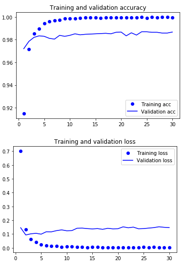
We still seem to be overfitting, suggesting we could potentially improve performance. The params on the top dense layers were fairly arbitrarily for this post. I'll leave improving performance further as an exercise for the reader. We've also trained on just 16,000 of the 25,000 images available. If the contest was still going we could retrain with the additional 9k images and likely have better results.
Finally lets compare to the test set.
test_generator = test_datagen.flow_from_directory(
    test_dir,
    target_size=(224, 224),
    batch_size=50,
    class_mode='binary')

test_loss, test_acc = model.evaluate_generator(test_generator, steps=90)
print('test acc:', test_acc)
Found 4500 images belonging to 2 classes.
test acc: 0.9862222280767229
98.6% accuracy. Not bad at all, it goes to show how lucky we have it these days. This would have been competitive with a state of the art solution not that many years ago, and now we can achieve it with Keras and just a few lines of Python.