Cats vs Dogs - Part 1 - 92.8% Accuracy - Binary Image Classification with Keras and Deep Learning
May 07, 2019 -In 2014 Kaggle ran a competition to determine if images contained a dog or a cat. In this series of posts we'll see how easy it is to use Keras to create a 2D convolutional neural network that potentially could have won the contest.
We will start with a basic neural network that is 84% accurate at predicting whether an image contains a cat or dog. Then we'll add dropout and finally add data augmentation to get to 92.8% categorization accuracy.
In part 2 we'll see how we can fine tune a network pretrained on ImageNet and take advantage of transfer learning to reach 98.6% accuracy (the winning entry scored 98.9%).
In part 3 we'll switch gears and use PyTorch instead of Keras to create an ensemble of models that provides more predictive power than any single model and reaches 99.1% accuracy.
The code is available in a jupyter notebook here. You will need to download the data from the Kaggle competition. The dataset contains 25,000 images of dogs and cats (12,500 from each class). We will create a new dataset containing 3 subsets, a training set with 16,000 images, a validation dataset with 4,500 images and a test set with 4,500 images.
Build the first network
We'll use the Keras sequential API to build a pretty straightforward network that consists of a number of Conv2D and pooling layers with a dense network at the end that makes the cat or dog prediction.
from keras import layers, models, optimizers

model = models.Sequential()
model.add(layers.Conv2D(32, (3, 3), activation='relu', input_shape=(224, 224, 3)))
model.add(layers.MaxPool2D(2, 2))
model.add(layers.Conv2D(64, (3, 3), activation='relu'))
model.add(layers.MaxPool2D(2, 2))
model.add(layers.Conv2D(128, (3, 3), activation='relu'))
model.add(layers.MaxPool2D(2, 2))
model.add(layers.Conv2D(128, (3, 3), activation='relu'))
model.add(layers.MaxPool2D(2, 2))
model.add(layers.Flatten())
model.add(layers.Dense(512, activation='relu'))
model.add(layers.Dense(1, activation='sigmoid'))

model.compile(loss='binary_crossentropy',
              optimizer=optimizers.RMSprop(lr=1e-4),
              metrics=['acc'])
We'll create some generators that will do some preprocessing on the images and resize them to be 224x224 pixels.
from keras.preprocessing.image import ImageDataGenerator

# Rescale pixel values from [0, 255] to [0, 1]
train_datagen = ImageDataGenerator(rescale=1./255)
test_datagen = ImageDataGenerator(rescale=1./255)

# The list of classes will be automatically inferred from the subdirectory names/structure under train_dir
train_generator = train_datagen.flow_from_directory(
    train_dir,
    target_size=(224, 224), # resize all images to 224 x 224
    batch_size=50,
    class_mode='binary') # because we use binary_crossentropy loss we need binary labels

validation_generator = test_datagen.flow_from_directory(
    validation_dir,
    target_size=(224, 224),
    batch_size=50,
    class_mode='binary')
Found 16000 images belonging to 2 classes.
Found 4500 images belonging to 2 classes.
Now lets fit the network for 30 epochs.
history = model.fit_generator(
    train_generator,
    steps_per_epoch=320, # 50 batches in the generator, so it takes 320 batches to get to 16000 images
    epochs=30,
    validation_data=validation_generator,
    validation_steps=90) # 90 x 50 == 4500
Epoch 1/30
320/320 [==============================] - 48s 150ms/step - loss: 0.6070 - acc: 0.6579 - val_loss: 0.5263 - val_acc: 0.7413
Epoch 2/30
320/320 [==============================] - 45s 142ms/step - loss: 0.5145 - acc: 0.7433 - val_loss: 0.5812 - val_acc: 0.6971
...
...
...
Epoch 29/30
320/320 [==============================] - 46s 143ms/step - loss: 0.0133 - acc: 0.9959 - val_loss: 0.9195 - val_acc: 0.8349
Epoch 30/30
320/320 [==============================] - 46s 143ms/step - loss: 0.0133 - acc: 0.9965 - val_loss: 0.8704 - val_acc: 0.8351
Plotting the results (code to generate the graphs is available in the jupyter notebook) we can see that the model begins to overfit the training data almost immediately. The training accuracy continues to improve until it gets close to 100%, while the validation set tops out at around 84% and loss degrades as training continues.
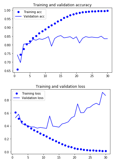
In the final epoch we reached 83.5% accuracy on the validation set, lets quickly double check on the test set to compare.
test_generator = test_datagen.flow_from_directory(
    test_dir,
    target_size=(224, 224),
    batch_size=50,
    class_mode='binary')

test_loss, test_acc = model.evaluate_generator(test_generator, steps=90)
print('test acc:', test_acc)
Found 4500 images belonging to 2 classes.
test acc: 0.8406666629844242
On one hand this isn't horrible, a baseline where we pick dog every time would have 50% accuracy. But on the other hand we can do much better.
Add Dropout
We can add dropout to regularize the model. Adding dropout randomly removes a percentage of neurons (sets their value to 0) at each update during training time, which helps prevent overfitting. By randomly throwing out data this will help to prevent the network from becoming too smart and essentially memorizing the training data, and thereby generalize to new data better.
from keras import layers, models, optimizers

model = models.Sequential()
model.add(layers.Conv2D(32, (3, 3), activation='relu', input_shape=(224, 224, 3)))
model.add(layers.MaxPool2D(2, 2))
model.add(layers.Conv2D(64, (3, 3), activation='relu'))
model.add(layers.MaxPool2D(2, 2))
model.add(layers.Conv2D(128, (3, 3), activation='relu'))
model.add(layers.MaxPool2D(2, 2))
model.add(layers.Conv2D(128, (3, 3), activation='relu'))
model.add(layers.MaxPool2D(2, 2))
model.add(layers.Flatten())
model.add(layers.Dropout(0.5)) # Note the only change is that we added dropout here
model.add(layers.Dense(512, activation='relu'))
model.add(layers.Dense(1, activation='sigmoid'))

model.compile(loss='binary_crossentropy',
              optimizer=optimizers.RMSprop(lr=1e-4),
              metrics=['acc'])
How does this model perform?
Epoch 1/30
320/320 [==============================] - 46s 145ms/step - loss: 0.6166 - acc: 0.6449 - val_loss: 0.5348 - val_acc: 0.7378
Epoch 2/30
320/320 [==============================] - 46s 143ms/step - loss: 0.5280 - acc: 0.7364 - val_loss: 0.4777 - val_acc: 0.7733
...
...
...
Epoch 29/30
320/320 [==============================] - 46s 144ms/step - loss: 0.1037 - acc: 0.9603 - val_loss: 0.3722 - val_acc: 0.8720
Epoch 30/30
320/320 [==============================] - 46s 144ms/step - loss: 0.1030 - acc: 0.9604 - val_loss: 0.3444 - val_acc: 0.8780
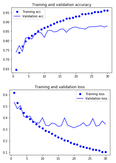
We still seem to be overfitting, but not as badly. We've also increase validation accuracy to 87.8%, so this is a bit of a win. We could try tuning the network architecture or the dropout amount, but instead lets try something else next.
Add Data Augmentation
Keras includes an ImageDataGenerator class which lets us generate a number of random transformations on an image. Since we're only training on 16,000 images, we can use this to create "new" images to help the network learn. There are limits to how much this can help, but in this case we will get a decent accuracy boost.
from keras.preprocessing.image import ImageDataGenerator

datagen = ImageDataGenerator(
    rotation_range=40,
    width_shift_range=0.2,
    height_shift_range=0.2,
    shear_range=0.2,
    zoom_range=0.2,
    horizontal_flip=True,
    fill_mode='nearest')
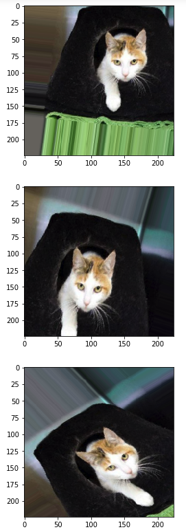
The above creates a data generator that will take in an image from the training set and return an image that has been slightly altered. Lets visualize what this looks like.
from keras.preprocessing import image

fnames = [os.path.join(train_cats_dir, fname) for fname in os.listdir(train_cats_dir)]
img_path = fnames[4] # Choose one image to augment
img = image.load_img(img_path, target_size=(224, 224)) # load image and resize it
x = image.img_to_array(img) # Convert to a Numpy array with shape (224, 224, 3)
x = x.reshape((1,) + x.shape)

# Generates batches of randomly transformed images.
# Loops indefinitely, so you need to break once three images have been created
i = 0
for batch in datagen.flow(x, batch_size=1):
    plt.figure(i)
    imgplot = plt.imshow(image.array_to_img(batch[0]))
    i += 1
    if i % 3 == 0:
        break
plt.show()
We'll use the same network architecture as the previous step, but generate images like this
train_datagen = ImageDataGenerator(
    rescale=1./255,
    rotation_range=40,
    width_shift_range=0.2,
    height_shift_range=0.2,
    shear_range=0.2,
    zoom_range=0.2,
    horizontal_flip=True)

test_datagen = ImageDataGenerator(rescale=1./255) # Note that validation data should not be augmented

train_generator = train_datagen.flow_from_directory(
    train_dir,
    target_size=(224, 224),
    batch_size=50,
    class_mode='binary')

validation_generator = test_datagen.flow_from_directory(
    validation_dir,
    target_size=(224, 224),
    batch_size=50,
    class_mode='binary')
Found 16000 images belonging to 2 classes.
Found 4500 images belonging to 2 classes.
And then increase the steps per epoch 3x so that we are training on 48,000 images instead of 16,000. This takes awhile as in the example I'm running on a 5 year old GPU I had laying around the house, training should be much faster if you can use more recent hardware or rent time on a GPU in the cloud.
history = model.fit_generator(
    train_generator,
    steps_per_epoch=960, # 960 x 50 = 48000 (we are showing different augmented images more than once per epoch)
    epochs=30,
    validation_data=validation_generator,
    validation_steps=90) # 90 x 50 == 4500
Epoch 1/30
960/960 [==============================] - 411s 429ms/step - loss: 0.6202 - acc: 0.6428 - val_loss: 0.5285 - val_acc: 0.7413
Epoch 2/30
960/960 [==============================] - 410s 427ms/step - loss: 0.5495 - acc: 0.7141 - val_loss: 0.5082 - val_acc: 0.7447
...
...
...
Epoch 29/30
960/960 [==============================] - 409s 426ms/step - loss: 0.2323 - acc: 0.9057 - val_loss: 0.2284 - val_acc: 0.9136
Epoch 30/30
960/960 [==============================] - 413s 430ms/step - loss: 0.2330 - acc: 0.9040 - val_loss: 0.1821 - val_acc: 0.9222
And finally compare to the holdout test set.
test_generator = test_datagen.flow_from_directory(
    test_dir,
    target_size=(224, 224),
    batch_size=50,
    class_mode='binary')

test_loss, test_acc = model.evaluate_generator(test_generator, steps=90)
print('test acc:', test_acc)
Found 4500 images belonging to 2 classes.
test acc: 0.928444442484114
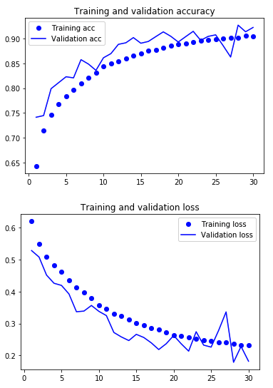
Yet another improvement, we've reached 92.8% on the test set, are seeing similar numbers on the validation data, and overfitting doesn't seem to be nearly as much of a problem.
We could work to improve these results, but that's all for today. In the next post we’ll see how we can take advantage of transfer learning to reach 98.6% accuracy.